7.4 Systematic Sampling • Systematic sampling is a sampling plan in

7.4 Systematic Sampling

• Systematic sampling is a sampling plan in which the population units are collected

systematically throughout the population. More speciﬁcally, a single primary sampling

unit consists of secondary sampling units that are relatively spaced with each other in

some systematic pattern throughout the population.

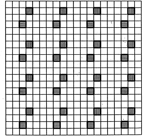
• Supp ose the study area is partitioned into a 20 × 20 grid of 400 population units. A

primary sampling unit in a systematic sample could consist of all population units that

form a lattice which are 5 units apart horizontally and vertically. In Figure 9a, N = 25

and M = 16. In Figure 9b, each of the N = 50 primary sampling units contains M = 8

secondary sampling units.

• Initially, systematic sampling and cluster sampling appear to be opposites because system-

atic samples contain secondary sampling units that are spread throughout the population

(go od global coverage of the study area) while cluster samples are collected in groups of

close proximity (good coverage locally within the study area).

• Systematic and cluster sampling are similar, however, because whenever a primary sam-

pling unit is selected from the sampling frame, all secondary sampling units of that primary

sampling unit will be included in the sample. Thus, random selection occurs at the primary

sampling unit level and not the secondary sampling unit level.

• For estimation purposes, you could ignore the secondary sampling unit y

-values and only

retain the primary sampling units t

-values. This is what we did with one-stage cluster

sampling.

• The systematic and cluster sampling principle: To obtain estimators of low variance,

the population must be partitioned into primary sampling unit clusters in such a way that

157

7.4 Systematic Sampling

• Systematic sampling is a sampling plan in which the population units are collected

systematically throughout the population. More speciﬁcally, a single primary sampling

unit consists of secondary sampling units that are relatively spaced with each other in

some systematic pattern throughout the population.

• Suppose the study area is partitioned into a 20 × 20 grid of 400 population units. A

primary sampling unit in a systematic sample could consist of all population units that

form a lattice which are 5 units apart horizontally and vertically. In Figure 9a, N = 25

and M = 16. In Figure 9b, each of the N = 50 primary sampling units contains M = 8

secondary sampling units.

• Initially, systematic sampling and cluster sampling appear to be opposites because system-

atic samples contain secondary sampling units that are spread throughout the population

(good global coverage of the study area) while cluster samples are collected in groups of

close proximity (good coverage locally within the study area).

• Systematic and cluster sampling are similar, however, because whenever a primary sam-

pling unit is selected from the sampling frame, all secondary sampling units of that primary

sampling unit will be included in the sample. Thus, random selection occurs at the primary

sampling unit level and not the secondary sampling unit level.

• For estimation purposes, you could ignore the secondary sampling unit y

-values and only

retain the primary sampling units t

-values. This is what we did with one-stage cluster

sampling.

• The systematic and cluster sampling principle: To obtain estimators of low variance,

the population must be partitioned into primary sampling unit clusters in such a way that

the clusters are similar to each other with respect to the t

-values (small cluster-to-cluster

variability).

161

• This is equivalent to saying that the within-cluster variability should be as large as pos-

sible to obtain the most precise estimators. Thus, the ideal primary sampling unit is

representative of the full diversity of y

-values within the population.

• With natural populations of spatially distributed plants, animals, minerals, etc., these con-

ditions are typically satisﬁed by systematic primary sampling units (and are not satisﬁed

by primary sampling units with spatially clustered secondary sampling units).

7.4.1 Estimation of y

and t

• If a SRS is used to select the systematic primary sampling units, we can apply the estima-

tion results for cluster sampling to deﬁne (i) estimators, (ii) the variance of each estimator,

and (iii) the estimated variance of each estimator.

• The following formulas will be the same as those used for one-stage cluster sampling. The

subscript sys denotes the fact that data were collected under systematic sampling.

• The unbiased estimators of t and y

are:

sys

i=1

sys

i=1

= (85)

with variance

V (

sys

) = V (

sys

) =

N(N −n)

(86)

where S

i=1

− t

)

N −1

• Recall that y =

i=1

is the sample mean and that s

i=1

− y)

n −1

is the sample

variance of the primary sampling units.

• Because S

is unknown, we use s

to get unbiased estimators of the variances:

V (

sys

) =

V (

sys

) =

N(N −n)

(87)

7.4.2 Conﬁdence Intervals for y

and t

• For a relatively small number n of sampled primary sampling units, the following conﬁ-

dence intervals are recommended:

sys

± t

∗

V (

sys

)

sys

± t

∗

V (

sys

) (88)

where t

∗

is the upper α/2 critical value from the t(n − 1) distribution. Note that the

degrees of freedom are based on n, the number of sampled primary sampling units, and

not on the total number of secondary sampling units nM.

162

Systematic Sampling Examples

In Figure 9a, each of the N = 25 primary sampling units contains M = 16 secondary sampling

units corresponding to the same location within the 16 5x5 subregions. n = 3 primary sampling

units were sampled. The SSUs sampled are in ( )

Figure 9a

1 1 (1) 1 1 2 1 (0) 0 0 4 5 (0) 1 0 1 2 (1) 0 1

3 2 1 0 1 0 0 0 1 2 2 2 0 2 2 2 0 2 0 1

7 (4) 1 1 1 1 (0) 0 0 2 2 (0) 4 3 2 4 (2) 1 2 2

0 1 2 0 0 0 0 0 4 6 5 1 5 0 0 0 2 1 2 0

1 1 0 (2) 3 2 0 0 (2) 1 3 1 4 (1) 1 1 2 2 (1) 1

2 0 (0) 0 4 3 3 (0) 1 16 5 0 (1) 3 8 0 0 (1) 3 3

0 0 1 14 3 3 1 2 0 8 0 2 0 3 9 0 4 2 1 0

0 (0) 5 1 8 7 (6) 6 6 1 0 (4) 0 0 1 2 (2) 0 1 2

0 0 2 2 3 2 2 3 1 1 1 3 0 0 2 2 0 3 4 0

0 0 0 (0) 1 0 3 1 (1) 1 2 0 2 (0) 2 0 2 1 (1) 0

1 8 (7) 7 8 0 5 (0) 1 0 1 2 (0) 0 2 4 2 (2) 2 4

0 9 1 0 0 1 1 1 0 0 0 1 2 4 0 2 1 3 3 1

0 (0) 0 1 0 2 (4) 3 1 2 2 (0) 0 1 1 2 (2) 0 2 4

0 1 0 0 1 2 0 2 3 5 2 0 0 2 1 1 2 0 1 3

1 0 0 (1) 1 0 0 0 (2) 2 2 1 1 (1) 0 0 2 0 (0) 0

0 2 (0) 2 2 0 1 (1) 0 2 0 0 (1) 0 0 1 1 (1) 5 3

0 0 0 3 2 1 0 0 0 0 0 2 1 0 1 1 1 3 1 2

1 (0) 0 1 0 3 (0) 1 0 0 2 (1) 2 0 0 0 (1) 1 1 0

0 0 0 0 0 0 0 1 1 1 0 1 0 3 0 2 0 1 1 0

2 0 0 (0) 0 0 0 0 (1) 2 0 1 3 (0) 0 1 0 1 (2) 4

The following are the 25 systematic PSU (cluster) totals (t

for i = 1, 2, . . . , 25). The sample

contains n = 3 PSU (3 starting locations). The PSUs sampled are in ( )

25 33 (16) 26 54

15 26 19 32 32

35 (26) 24 21 26

17 13 20 24 23

15 13 15 (15) 19

163

In Figure 9b, each of the N = 50 primary sampling units contains M = 8 secondary sampling

units corresponding to the same location within the 8 10x5 subregions. n = 6 primary sampling

units were sampled. The SSUs sampled are in ( )

Figure 9b

18 (20) 15 20 20 15 (19) 18 24 23 20 (26) 29 28 28 31 (31) 34 28 32

13 20 16 20 15 23 19 26 21 21 24 30 23 26 25 33 31 28 32 38

(16) 18 20 24 (25) (26) 22 23 26 (26) (22) 27 25 25 (34) (28) 37 36 38 (31)

17 17 16 22 21 23 22 27 27 24 28 32 29 33 27 37 37 38 35 33

15 19 23 17 21 23 21 23 24 25 31 26 32 34 32 33 31 31 36 37

21 (24) 20 21 28 26 (30) 22 31 25 29 (29) 27 30 29 37 (35) 32 38 43

23 17 24 25 24 27 31 29 31 34 27 36 29 29 34 39 37 37 40 36

(18) 24 21 25 27 (22) 32 32 31 26 (28) 34 34 37 35 (34) 38 38 37 40

22 26 28 (26) 24 29 33 26 (27) 27 34 31 39 (32) 36 38 37 40 (44) 43

23 27 28 29 26 32 25 31 35 34 32 33 37 32 42 40 40 37 42 44

23 (21) 31 23 30 27 (31) 30 32 35 30 (40) 32 37 37 36 (40) 44 44 40

26 29 31 26 30 31 34 36 30 38 36 32 38 38 37 42 42 41 40 49

(28) 24 28 27 (26) (31) 32 29 32 (33) (38) 34 39 38 (40) (37) 41 43 42 (43)

32 25 31 32 29 29 35 38 38 32 36 35 39 42 39 40 44 42 41 45

27 29 35 28 35 35 31 40 35 37 38 44 40 40 47 39 49 48 51 49

30 (29) 32 32 33 30 (36) 38 42 36 35 (38) 44 47 45 49 (41) 43 44 51

28 35 35 34 34 33 41 33 34 35 39 44 44 48 44 50 49 48 53 54

(29) 33 32 36 39 (33) 33 34 35 42 (46) 47 48 47 46 (45) 44 52 54 55

28 37 38 (37) 33 33 34 37 (45) 40 39 42 42 (46) 47 48 52 47 (46) 53

38 39 39 37 34 38 39 45 39 42 45 41 44 51 46 50 52 51 51 53

The following are the 50 systematic PSU (cluster) totals (t

for i = 1, 2, . . . , 50). The sample

contains n = 6 PSU (6 starting locations). The PSUs sampled are in ( )

200 (228) 233 236 245

228 237 239 233 253

(226) 235 243 252 (258)

242 247 260 270 250

241 250 272 265 283

257 (262) 258 285 290

266 290 279 294 295

(255) 285 291 302 310

271 292 297 (303) 303

298 296 312 316 321

164

7.4.3 Using R and SAS for Systematic Sampling

R code for Systematic Sample in Figure 9a

library(survey)

source("c:/courses/st446/rcode/confintt.r")

# Systematic sample of 3 PSUs from Figure 9a

N = 25

n = 3

M = 16

wgt = N/n

y <- c(1,0,0,1,0,0,1,1,7,0,0,2,0,1,1,1,

4,0,0,2,0,6,4,2,0,4,0,2,0,0,1,1,

2,2,1,1,0,1,0,1,1,2,1,0,0,1,0,2)

clusterid <- c(rep(c(1),M),rep(c(2),M),rep(c(3),M))

fpc <- c(rep(N,n*M))

Fig9a <- data.frame(cbind(clusterid,y,fpc))

dsgn9a <-

svydesign(ids=~clusterid,weights=c(rep(wgt,n*M)),fpc=~fpc,data=Fig9a)

esttotal <- svytotal(~trees,design=dsgn9a)

print(esttotal,digits=15)

confint.t(esttotal,level=.95,tdf=n-1)

estmean <- svymean(~trees,design=dsgn9a)

print(estmean,digits=15)

confint.t(estmean,level=.95,tdf=n-1)

R output for Systematic Sample in Figure 9a

total SE

y 475 82.361

-------------------------------------------------------------------

mean( y ) = 475.00000

SE( y ) = 82.36099

Two-Tailed CI for y where alpha = 0.05 with 2 df

2.5 % 97.5 %

120.62924 829.37076

-------------------------------------------------------------------

mean SE

y 1.1875 0.2059

-------------------------------------------------------------------

mean( y ) = 1.18750

SE( y ) = 0.20590

Two-Tailed CI for y where alpha = 0.05 with 2 df

2.5 % 97.5 %

0.30157 2.07343

-------------------------------------------------------------------

165

R code for Systematic Sample in Figure 9b

# Systematic sample of 6 PSUs from Figure 9b

N = 50

n = 6

M = 8

wgt = N/n

y <- c(20,19,26,31,21,31,40,40,16,26,22,28,28,31,38,37,

25,26,34,31,26,33,40,43,24,30,29,35,29,36,38,41,

18,22,28,34,29,33,46,45,26,27,32,44,37,45,46,46)

clusterid <- c(1,1,1,1,1,1,1,1,2,2,2,2,2,2,2,2,3,3,3,3,3,3,3,3,

4,4,4,4,4,4,4,4,5,5,5,5,5,5,5,5,6,6,6,6,6,6,6,6)

(The remainder of the code is the same as the previous example)

R output for Systematic Sample in Figure 9b

-------------------------------------------------------------------

mean( y ) = 12766.66667

SE( y ) = 536.93368

Two-Tailed CI for y where alpha = 0.05 with 5 df

2.5 % 97.5 %

11386.43470 14146.89863

-------------------------------------------------------------------

mean( y ) = 31.91667

SE( y ) = 1.34233

Two-Tailed CI for y where alpha = 0.05 with 5 df

2.5 % 97.5 %

28.46609 35.36725

-------------------------------------------------------------------

SAS code for Systematic Sample in Figure 9a (Supplemental)

DATA systmtc1;

M0 = 400; * number of secondary sampling units (SSUs) in population;

M = 16; * number of SSUs in a PSU;

n = 3; * number of primary sampling units (PSUs) sampled;

wgt = M0/(n*M);

DO psu = 1 to n;

DO ssu = 1 to M;

INPUT trees @@; OUTPUT;

END; END;

DATALINES;

1 0 0 1 0 0 1 1 7 0 0 2 0 1 1 1

4 0 0 2 0 6 4 2 0 4 0 2 0 0 1 1

2 2 1 1 0 1 0 1 1 2 1 0 0 1 0 2

;

*** TOTAL = number of PSUs in the population ***;

PROC SURVEYMEANS DATA=systmtc1 TOTAL=25 MEAN CLM SUM CLSUM;

VAR trees;

CLUSTER psu;

WEIGHT wgt;

TITLE ’Systematic Sample from Figure 9a’;

RUN;

166

SAS output for Systematic Sample in Figure 9a

The SURVEYMEANS Procedure

Data Summary

Number of Clusters 3

Number of Observations 48

Sum of Weights 400

Statistics

Std Error

Variable Mean of Mean 95% CL for Mean

-----------------------------------------------------------------

trees 1.187500 0.205902 0.30157311 2.07342689

-----------------------------------------------------------------

Statistics

Variable Sum Std Dev 95% CL for Sum

-----------------------------------------------------------------

trees 475.000000 82.360994 120.629244 829.370756

-----------------------------------------------------------------

SAS code for Systematic Sample in Figure 9b (Supplemental)

DATA systmtc2;

M0 = 400; * number of secondary sampling units (SSUs) in population;

n = 6; * number of primary sampling units (PSUs) sampled;

m = 8; * number of SSUs in a PSU;

wgt = M0/(n*m);

DO psu = 1 to n; DO ssu = 1 to m;

INPUT y @@; OUTPUT;

END; END;

DATALINES;

20 19 26 31 21 31 40 40 16 26 22 28 28 31 38 37 25 26 34 31 26 33 40 43

24 30 29 35 29 36 38 41 18 22 28 34 29 33 46 45 26 27 32 44 37 45 46 46

;

*** TOTAL = number of PSUs in the population ***;

PROC SURVEYMEANS DATA=systmtc2 TOTAL=50 MEAN CLM SUM CLSUM;

VAR y; CLUSTER psu; WEIGHT wgt;

TITLE ’Systematic Sample from Figure 9b’;

RUN;

SAS output for Systematic Sample in Figure 9b

Data Summary

Number of Clusters 6

Number of Observations 48

Sum of Weights 400

Statistics

Std Error

Variable Mean of Mean 95% CL for Mean

-----------------------------------------------------------------

y 31.916667 1.342334 28.4660867 35.3672466

-----------------------------------------------------------------

Variable Sum Std Dev 95% CL for Sum

-----------------------------------------------------------------

y 12767 536.933681 11386.4347 14146.8986

-----------------------------------------------------------------

167

7.4.4 Comments from W.G. Cochran

• Cochran (from Sampling Techniques (1953)) makes the following comments about advan-

tages of systematic sampling:

Intuitively, systematic sampling seems likely to be more precise than simple random

sampling. In eﬀect, it stratiﬁes the population into [N] strata, which consist of the ﬁrst

[M] units, the second [M ] units, and so on. We might therefore expect the systematic

sample to be about as precise as the corresponding stratiﬁed random sample with

one unit per stratum. The diﬀerence is that with the systematic sample the units all

occur at the same relative position in the stratum, whereas with the stratiﬁed random

sample the position in the stratum is determined separately by randomization within

each stratum. The systematic sample is spread more evenly over the population, and

this fact has sometimes made systematic sampling considerably more precise than

stratiﬁed random sampling.

• Cochran also warns us that:

The performance of systematic sampling relative to that of stratiﬁed or simple random

sampling is greatly dependent on the properties of the population. There are popu-

lations for which systematic sampling is extremely precise and others for which it is

less precise that simple random sampling. For some populations and values of [M ],

[ var(

sys

)] may even increase when a larger sample is taken — a startling departure

from good behavior. Thus it is diﬃcult to give general advice about the situation in

which systematic sampling is to recommended. A knowledge of the structure of the

population is necessary for its most eﬀective use.

• If a population contains a linear trend:

1. The variances of the estimators from systematic and stratiﬁed sampling will be smaller

than the variance of the estimator from simple random sampling.

2. The variance of the estimator from systematic sampling will be larger than the vari-

ance of the estimator from stratiﬁed sampling. Why? If the starting point of the

systematic sample is selected too low or too high, it will be too low or too high

across the population of units. Whereas, stratiﬁed sampling gives an opportunity for

within-stratum errors to cancel.

• Suppose a population has 16 secondary sampling units (t = 130) and is ordered as follows:

Sampling unit 1 2 3 4 5 6 7 8 9 10 11 12 13 14 15 16

y-value 1 2 2 3 3 4 5 6 8 9 12 13 14 15 16 17

Note there is a linearly increasing trend in the y-values with the order of the sampling

units. Suppose we take a 1-in-4 systematic sample. The following table summarizes the

four possible 1-in-4 systematic samples.

Sampling unit 1 2 3 4 5 6 7 8 9 10 11 12 13 14 15 16

y-values 1 2 2 3 3 4 5 6 8 9 12 13 14 15 16 17 t

sys

Sample 1 1 3 8 14

Sample 2 2 4 9 15

Sample 3 2 5 12 16

Sample 4 3 6 13 17

168

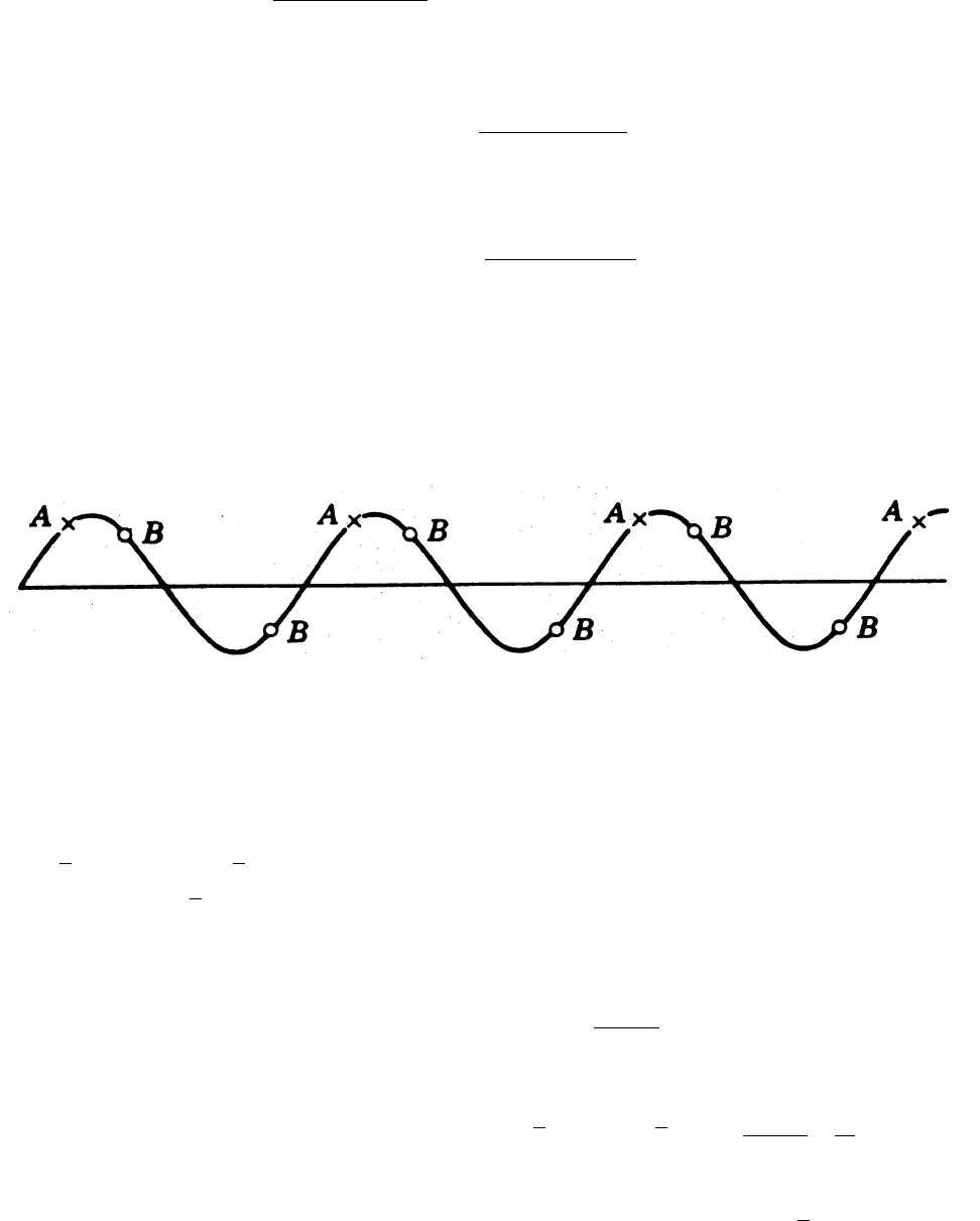
• If a population has periodic trends, the eﬀectiveness of the systematic sample depends

on the relationship between the periodic interval and the systematic sampling interval or

pattern. The following idealized curve was given by Cochran to show this. The height of

the curve represents the population y-value.

– The A sample points represent the least favorable systematic sample because when-

ever M is equal to the period, every observation in the systematic sample will be

similar so the sample is no more precise than a single observation taken at random

from the population.

– The B sample points represent the most favorable systematic sample because M is

equal to a half-period. Every systematic sample has mean equal to the true population

mean because successive y-value deviations above and below the mean cancel. Thus,

the variance of the estimator is zero.

– For other values of M, the sample has varying degrees of eﬀectiveness that depends

on the relation between M and the period.

• If a population has periodic trends, the eﬀectiveness of the systematic sample depends

on the relationship between the periodic interval and the systematic sampling interval or

pattern. The following idealized curve was given by Cochran to show this. The height of

the curve represents the population y-value.

– The A sample points represent the least favorable systematic sample because when-

ever M is equal to the period, every observation in the systematic sample will be

similar so the sample is no more precise than a single observation taken at random

from the population.

– The B sample points represent the most favorable systematic sample because M is

equal to a half-period. Every systematic sample has mean equal to the true population

mean because successive y-value deviations above and below the mean cancel. Thus,

the variance of the estimator is zero.

– For other values of M, the sample has varying degrees of eﬀectiveness that depends

on the relation between M and the period.

7.5 Using a Single Systematic Sample

• Many studies generate data from a systematic sample based on a single randomly selected

starting unit (i.e., there is only one randomly selected primary sampling unit).

• When there is only one primary sampling unit, it is possible to get unbiased estimators

sys

and

sys

of y

and t. It is not possible, however, to get an unbiased estimator of the

variances

V (

sys

) and

V (

sys

• If we can ignore the fact that the y

-values were collected systematically and treat the

M secondary sampling units in the single primary sampling unit as a SRS, then the SRS

variance estimator would be a reasonable substitute only if the units of the population can

reasonably be conceived as being randomly ordered (i.e., there is no systematic pattern in

the population such as a linear trend or a periodic pattern).

– If this assumption is reasonable, then

V (

sys

) ≈

V (

) =

N − n

• With natural populations in which nearby units are similar to each other (spatial correla-

tion), this procedure tends to provide overestimates of the variances of

sys

and

sys

• Procedures for estimating variances from a single systematic sample are discussed in Bell-

house (1988), Murthy and Rao (1988), and Wolter (1984).

165

7.5 Using a Single Systematic Sample

• Many studies generate data from a systematic sample based on a single randomly selected

starting unit (i.e., there is only one randomly selected primary sampling unit).

• When there is only one primary sampling unit, it is possible to get unbiased estimators

sys

and

sys

of y

and t. It is not possible, however, to get an unbiased estimator of the

variances

V (

sys

) and

V (

sys

• If we can ignore the fact that the y

-values were collected systematically and treat the

M secondary sampling units in the single primary sampling unit as a SRS, then the SRS

variance estimator would be a reasonable substitute only if the units of the population can

reasonably be conceived as being randomly ordered (i.e., there is no systematic pattern in

the population such as a linear trend or a periodic pattern).

– If this assumption is reasonable, then

V (

sys

) ≈

V (

) =



N −n



• With natural populations in which nearby units are similar to each other (spatial correla-

tion), this procedure tends to provide overestimates of the variances of

sys

and

sys

• Procedures for estimating variances from a single systematic sample are discussed in Bell-

house (1988), Murthy and Rao (1988), and Wolter (1984).

169