
1
Chapter 3: Simple Random Sampling and Systematic
Sampling
Simple random sampling and systematic sampling provide the foundation for almost all of the
more complex sampling designs that are based on probability sampling. They are also usually
the easiest designs to implement. These two designs highlight a trade-off inherent in all sampling
designs: do we select sample units at random to minimize the risk of introducing biases into the
sample or do we select sample units systematically to ensure that sample units are well-
distributed throughout the population?
Both designs involve selecting n sample units from the N units in the population and can be
implemented with or without replacement.
Simple Random Sampling
When the population of interest is relatively homogeneous then simple random sampling works
well, which means it provides estimates that are unbiased and have high precision. When little is
known about a population in advance, such as in a pilot study, simple random sampling is a
common design choice.
Advantages
:
• Easy to implement
• Requires little advance knowledge about the target population
Disadvantages
:
• Imprecise relative to other designs if the population is heterogeneous
• More expensive to implement than other designs if entities are clumped and the cost to
travel among units is appreciable
How it is implemented
:
• Select n sample units at random from N available in the population
All units within the population must have the same probability of being selected, therefore each
and every sample of size n drawn from the population has an equal chance of being selected.
There are many strategies available for selecting a
random sample. For large finite populations (i.e.,
those where every potential sampling unit can be
identified in advance), this can involve generating
pseudorandom numbers with a computer. For small
finite populations it might involve using a table of
random numbers or even writing a unique identifier for
every sample unit in the population on a scrap of
paper, placing those numbers in a jar, shaking it, then
selecting n scraps of paper from the jar blindly. The
approach used for selecting the sample matters little
provided there are no constraints on how the sample
units are selected and all units have an equal chance
of being selected.
2
Estimating the Population Mean
The population mean (μ) is the true average number of entities per sample unit and is estimated
with the sample mean (
μ
ˆ
or y ) which has an unbiased estimator:
n
y
n
i
i
∑
=
=
1
μ
ˆ
where y
i
is the value from each unit in the sample and n is the number of units in the sample.
The population variance (σ
2
) is estimated with the sample variance (s
2
) which has an unbiased
estimator:
1
1
2
2
−
−
=
∑
=
n
yy
s
n
i
i
)(
Variance of the estimate
μ
ˆ
is:
n
s
N
nN
)μ(
2
⎟
⎠
⎞
⎜
⎝
⎛
−
=
ˆ
ra
ˆ
v
.
The standard error of the estimate is the square root of variance of the estimate, which as always,
is the standard deviation of the sampling distribution of the estimate. Standard error is a useful
gauge of how precisely a parameter has been estimated as is a function of the variation inherent
in the population (σ
2
) and the size of the sample (n).
Standard error of
μ
ˆ
is:
n
s
N
nN
)μSE(
2
⎟
⎠
⎞
⎜
⎝
⎛
−
=
ˆ
.
The quantity
⎟
⎠
⎞
⎜
⎝
⎛
−
N
nN
is the finite population correction factor which adjusts variance of the
estimator (not variance of the population which does not change with n) to reflect the amount of
information that is known about the population through the sample. Simply, as the amount of
information we know about the population through sampling increases, the remaining uncertainty
decreases. Therefore, the correction factor reflects the proportion of the population that remains
unknown. Consequently, as the number of sampling units measured (n) approaches the total
number of sampling units in the population
(N), the finite population correction factor
approaches zero, so the amount of
uncertainty in the estimate also
approaches zero.
When the sample size n is small relative to
the population size N, the fraction of the
population being sampled n/N also is
small, therefore the correction factor has
little effect on the variance of the estimator
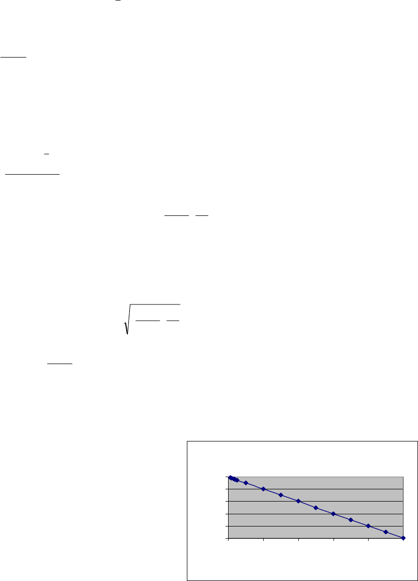
(Fig. 2 - FPC.xls). If the finite population
correction factor is ignored, which is what
FPC with N = 100
0
0.2
0.4
0.6
0.8
1
0 20406080100
n
FPC

3
we have to do when N is unknown, the effect on the variance of the estimator is slight when N is
large. When N is small, however, the variance of the estimator can be overestimated
appreciably.
Example
. (to be added)
Estimating the Population Total
Like the number of entities per sample unit, the total number of entities in the entire population is
another attribute estimated commonly. Unlike the population mean, however, estimating the
population total requires that we know the number of sampling units in a population, N.
The population total
∑
=
==
N
i
i
Ny
1
μτ
is estimated with the sample total (
τ
ˆ
) which has an unbiased
estimator:
∑
=
==
n
i
i
y
n
N
N
1
μτ
ˆˆ
where N is the total number of sample units in a population, n is the number of units in the
sample, and y
i
is the value measured from each sample unit.
In studies of wildlife populations, the total number of entities in a population is often referred to as
“abundance” and is traditionally represented with the symbol N. Consequently, there is real
potential for confusing the number of entities in the population with the number of sampling units
in the sampling frame. Therefore, in the context of sampling theory, we’ll use
τ
ˆ
to represent the
population total and N to represent the number of sampling units in a population. Later, when
addressing wildlife populations specifically, we’ll use N to represent abundance to remain
consistent with the literature in that field.
Because the estimator
τ
ˆ
is simply the number of sample units in the population N times the
mean number of entities per sample unit,
μ
ˆ
, the variance of the estimate
τ
ˆ
reflects both the
number of units in the sampling universe N and the variance associated with
μ
ˆ
. An unbiased
estimate for the variance of the estimate
τ
ˆ
is:
⎟
⎠
⎞
⎜
⎝
⎛
−
⎟
⎟
⎠
⎞
⎜
⎜
⎝
⎛
==
N
nN
n
s
NN
2
22
)
ˆ
var()
ˆ
var(
μτ
where s
2
is the estimated population variance.
Example
. (to be added)
Estimating a Population Proportion
If you are interested in the composition of a population, you could use a simple random sample to
estimate the proportion of the population p that is composed of elements with a particular trait,
such as the proportion of plants that flower in a given year, the proportion of juvenile animals
captured, the proportion of females in estrus, and so on. We will consider only classifications that
are dichotomous, meaning that an element in the population either has the trait of interest
(flowering) or it does not (not flowering); extending this idea to more complex classifications is
straightforward.

4
In the case of simple random sampling, the population proportion follows the mean exactly; that
is, p = μ. If this idea is new to you, convince yourself by working through an example. Say we
generate a sample of size 10, where 4 entities have a value of 1 and 6 entities have a value of 0
(e.g., 1 = presence of a trait, 0 = absence of a trait). The proportion of entities in the sample with
the trait is 4/10 or 0.40 which is also equal to the sample mean, which = 0.40
([1+1+1+1+0+0+0+0+0+0]/10 = 4/10). Cosmic.
It follows that the population proportion (p) is estimated with the sample proportion (
p
ˆ
) which has
an unbiased estimator:
n
y
p
n
i
i
∑
=
==
1
μ
ˆˆ
.
Because we are dealing with dichotomous proportions (sample unit does or does not have the
trait), the population variance σ
2
is computed based on variance for a binomial which is the
proportion of the population with the trait (p) times the proportion that does not have that trait (1 –
p) or p(1 – p). The estimate of the population variance s
2
is: )
ˆ
1(
ˆ
pp
−
.
Variance of the estimate
p
ˆ
is:
1
1
1
2
−
−
⎟
⎠
⎞
⎜
⎝
⎛
−
=
−
⎟
⎠
⎞
⎜
⎝
⎛
−
=
n
)p(p
N
nN
n
s
N
nN
)p(
ˆˆ
ˆ
ra
ˆ
v
.
Standard error of
p
ˆ
is:
1
1
1
2
−
−
⎟
⎠
⎞
⎜
⎝
⎛
−
=
−
⎟
⎠
⎞
⎜
⎝
⎛
−
=
n
)p(p
N
nN
n
s
N
nN
)pSE(
ˆˆ
ˆ
.
Example
. (to be added)
Determining Sample Sizes
How many sample units should we measure from the population so that we have confidence that
parameters have been estimated adequately?
Determining how many sample units (n) to measure requires that we establish the degree of
precision that we require for the estimate we wish to generate; we denote a quantity B, the
desired bound of the error of estimation, which we define as the half-width of the confidence
interval we want to result around the estimate we will generate from the proposed sampling effort.
To establish the number of sample units to measure to estimate the population mean μ at a
desired level of precision B with simple random sampling, we set Z × SE(
y ) (the formula for a
confidence interval) equal to B and solve this expression for n. We use Z to denote the upper α/2
point of the standard normal distribution for simplicity (although we could use the Student’s t
distribution), where α is the same value we used to establish the width of a confidence interval,
the rate at which we are willing to tolerate Type I errors.
We set
⎟
⎟
⎠
⎞
⎜
⎜
⎝
⎛
⎟
⎟
⎠
⎞
⎜
⎜
⎝
⎛
−
=
n
σ
N
nN
ZB
2
and solve for n:

5
2
22
0
0
11
1
B
Z
n
Nn
n
σ
=
+
= ; .
If we anticipate n to be small relative to N, we can ignore the population correction factor and use
only the formula for n
0
to gauge sample size.
Example: Estimate the average amount of money μ for a hospital’s accounts receivable. Note,
however, that no prior information exists with which to estimate population variance σ
2
but we
know that most receivables lie within a range of about $100 and there are N = 1000 accounts.
How many samples are needed to estimate μ with a bound on the error of estimation B = $3 with
95% confidence (α = 0.05, Z = 1.96) using simple random sampling?
Although it is ideal to have data with which to estimate σ
2
, the range is often approximately equal
to 4 σ, so one-fourth of the range might be used as an approximate value of σ.
25
4
100
4
==≈
range
σ
Substituting into the formula above:
4217
0001000360
1
1000
1
78277
1
1
1000
1
3
25961
1
1
2
22
.
..
.
.
=
+
=
+
=
+
=n
Therefore, about 218 samples are needed to estimate μ with a bound on the error of estimation
B = $3.
To establish the number of sample units to measure to estimate the population total τ at a desired
level of precision B with simple random sampling, we set
⎟
⎟
⎠
⎞
⎜
⎜
⎝
⎛
−=
n
nNNZB
2
σ
)(
and solve for n:
2
222
0
0
11
1
B
ZN
n
Nn
n
σ
=
+
= ;
And as with establishing n for the population mean, if N is large relative to n, the population
correction factor can be ignored, and the formula for sample size reduced to n
0
Example: What sample size is necessary to estimate the caribou population we examined to
within d = 2000 animals of the true total with 90% confidence (α = 0.10)?
Using s
2
= 919 from earlier and Z = 1.645, which is the upper α = 0.10/2 = 0.05 point of the
normal distribution:
51
2000
9196451286
2
222
0
≈=
.
n .
To adjust for the size of the finite population:

6
.44
286
1
51
1
1
≈
+
=n
Systematic Sampling
Occasionally, selecting sample units at random can introduce logistical challenges that preclude
collecting data efficiently. If we suspect that the chances of introducing a bias are low or if ideal
dispersion of sample units throughout the population is a higher priority than minimizing potential
biases, then it might be most appropriate to choose samples non-randomly. As in simple random
sampling, systematic sampling is a type of probability sampling where each element in the
population has a known and equal probability of being selected. The probabilistic framework is
maintained through selection of one or more random starting points. Although sometimes more
convenient, systematic sampling does provide less protection against introducing biases in the
sample compared to simple random sampling.
Estimators for systematic sampling and simple random sampling are identical; only the method of
sample selection differs. Therefore, systematic sampling is used most often to simplify the
process of selecting a sample or to ensure ideal dispersion of sample units throughout the
population.
Advantages
:
• Easy to implement
• Maximum dispersion of sample units throughout the population
• Requires minimum knowledge of the population
Disadvantages
:
• Less protection from possible biases
• Can be imprecise and inefficient relative to other designs if the population being sampled
is heterogeneous
How it is implemented
:
• Choose a starting point at random
• Select samples at uniform intervals thereafter
1-in-k systematic sample
Most commonly, a systematic sample is obtained by
randomly selecting 1 unit from the first k units in the
population and every k
th
element thereafter. This
approach is called a 1-in-k systematic sample with a
random start. To choose k so than a sample of
appropriate size is selected, calculate:
k = Number of units in population / Number of sample
units required
For example, if we plan to choose 40 plots from a field
of 400 plots, k = 400/40 = 10, so this design would be

7
a 1-in-10 systematic sample. The example in the figure is a 1-in-8 sample drawn from a
population of N = 300; this yields n = 28. Note that the sample size drawn will vary and depends
on the location of the first unit drawn.
Estimating the Population Mean
The population mean (μ) is estimated with:
n
y
n
i
i
∑
=
=
1
μ
ˆ
The population variance (σ
2
) is estimated with:
1
1
2
2
−
−
=
∑
=
n
yy
s
n
i
i
)(
Variance of the estimate
μ
ˆ
is:
n
s
N
nN
2
⎟
⎠
⎞
⎜
⎝
⎛
−
=)
ˆ
r(a
ˆ
v
μ
.
Standard error of
μ
ˆ
is:
n
s
N
nN
SE
2
⎟
⎠
⎞
⎜
⎝
⎛
−
=)
ˆ
(
μ
.
Estimating the Population Total
The population total
τ
is estimated with:
∑
=
==
n
i
i
y
n
N
N
1
μτ
ˆˆ
.
Variance of the estimate
τ
ˆ
is:
⎟
⎠
⎞
⎜
⎝
⎛
−
⎟
⎟
⎠
⎞
⎜
⎜
⎝
⎛
==
N
nN
n
s
NN
2
22
)
ˆ
var()
ˆ
r(a
ˆ
v
μτ
.
Standard error of
τ
ˆ
is:
⎟
⎠
⎞
⎜
⎝
⎛
−
⎟
⎟
⎠
⎞
⎜
⎜
⎝
⎛
=
N
nN
n
s
N
2
2
)
ˆ
r(a
ˆ
v
τ
Estimating the Population Proportion
The population proportion (p) is estimated with the sample proportion ( p
ˆ
) which has an unbiased
estimator:
n
y
p
n
i
i
∑
=
==
1
μ
ˆˆ
.
Because we are estimating a dichotomous proportion, the population variance σ
2
is again
computed with a binomial which is the proportion of the population with the trait (p) times the
proportion without that trait (1 – p) or p(1 – p). The estimate of the population variance s
2
is:
)
ˆ
(
ˆ
pp −1 .

8
Variance of the estimate
p
ˆ
is:
1
1
1
2
−
−
⎟
⎠
⎞
⎜
⎝
⎛
−
=
−
⎟
⎠
⎞
⎜
⎝
⎛
−
=
n
pp
N
nN
n
s
N
nN
p
)
ˆ
(
ˆ
)
ˆ
r(a
ˆ
v
.
Examples
. (to be added)
